Getting started with R

Session 1 of 4: The basics

Freddie Heather

We have a problem

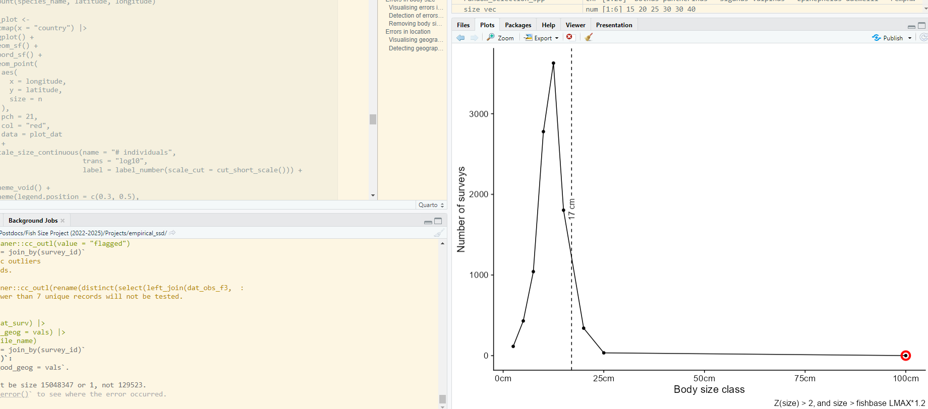
Problem: We are given an excel file with 1M+ rows, with species names, latitude and longitude of occurrence, and we must find errors in a species geographical distribution. The analysis is complicated and involves multiple steps that need to be replicated by others in the future.

Solution: R

Today’s workshop

We will work through the slides and problems together
This session is interactive. Please stop me and ask questions.
By the end of today: you will have learnt how to read in excel data into R, perform import checks, understand R programming basics.
Tips: be curious, play around, and try and break R (get some Errors)

The background of R

What is R?

Programming language
Very popular in scientific data analysis…
and a lot more

R is a tool

	Mechanics	Science
Problem	Bolt won’t loosen by hand	I have hypothesis and data; I want results for a paper
Solution	Use a spanner/wrench/socket/hammer	Use functions in R to import, clean, visualise and model data
Outcome	Loosen bolt	Figures and statistics

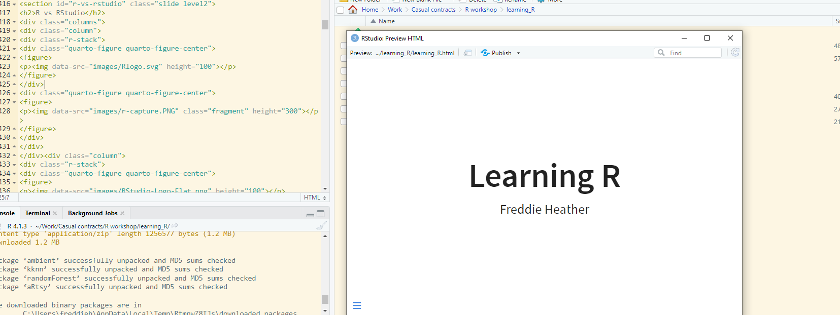
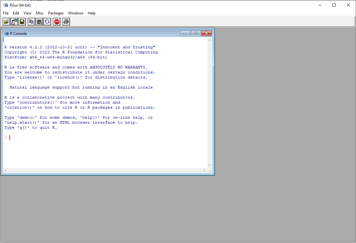
R vs RStudio

The coding language
(think car engine)
Download it and forget about it

User interface
(think car dashboard)
Open this when you want to code

Downloading R and RStudio

R: cran.r-project.org
RStudio: posit.co/download/rstudio-desktop

Let’s code!

Starting a new analysis

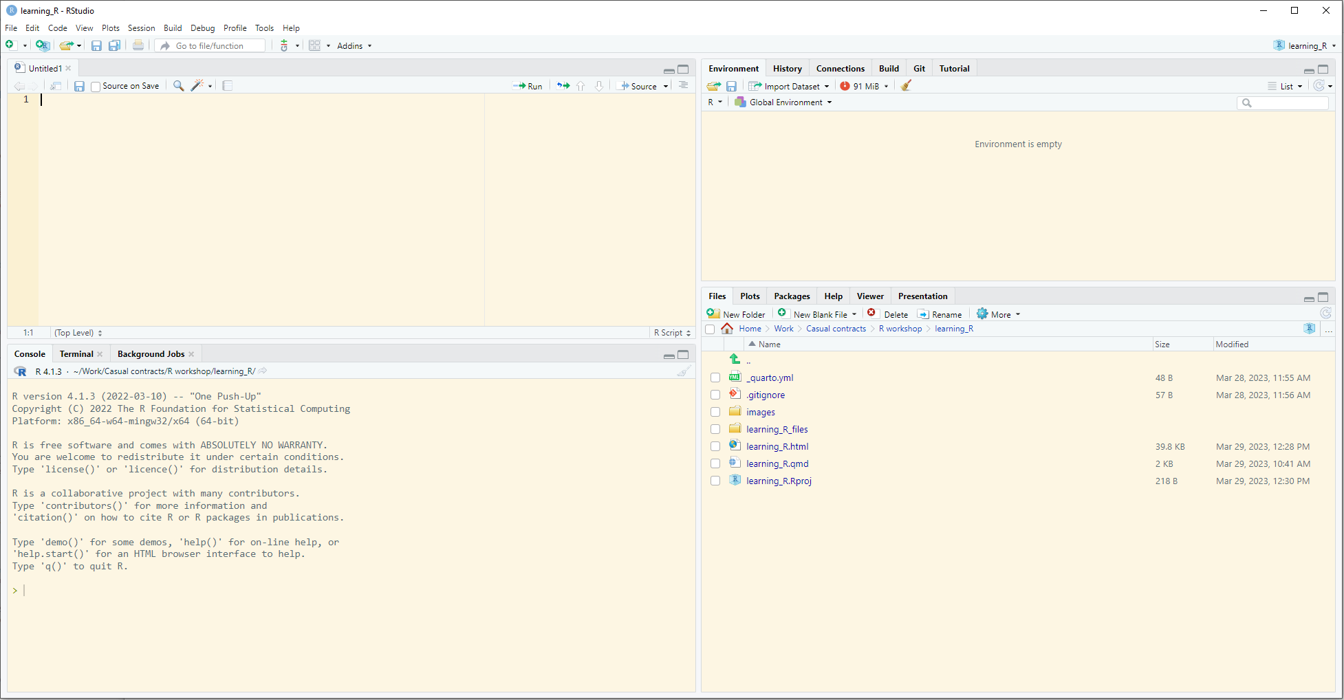
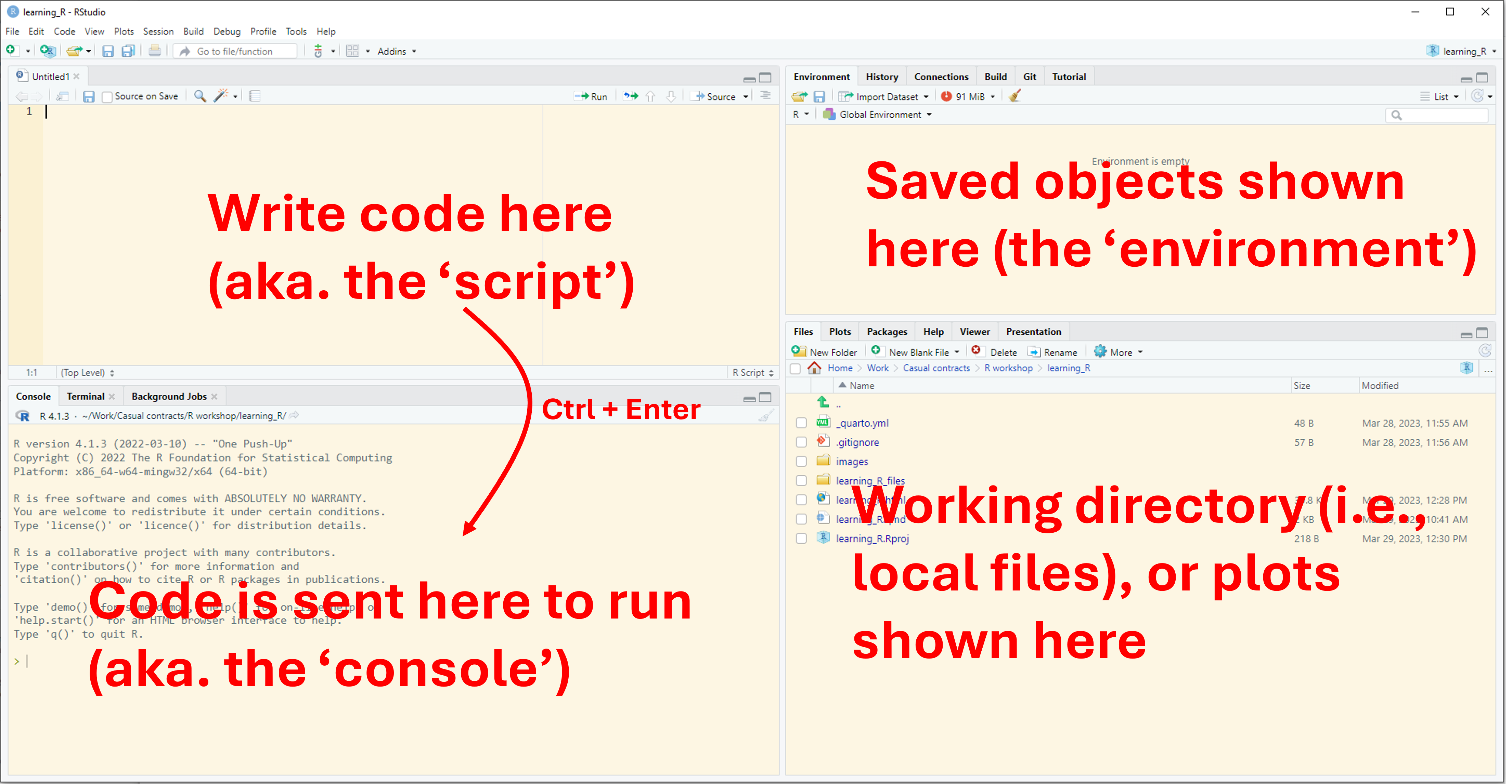
Opening R Studio

R projects

The key to organisational sucess

Similar to folders on your computers
R knows exactly where to look for things

Task: Start a new R project - Open RStudio - New Project - New Directory > New Project - Browse location for location of all R projects - Give a good title for the analysis (e.g. “phd_chapter_1”) - avoid spaces and capitals

Creating reproducible code (a script)

File > New file > R Script
Write anything (e.g. a comment with your name or title on line 1)
Save As “analysis.R”

Basic commands

# addition
# numeric output
1 + 3

[1] 4

# numeric vector (i.e. a series of numbers)
1:5

[1] 1 2 3 4 5

# or
c(1, 2, 3, 4, 5)

[1] 1 2 3 4 5

# Arithmetic on a vector
(1:5) * 2

[1]  2  4  6  8 10

Objects

An “object” can be anything: a number, a word, a plot, an equation, etc.
The code to create an object is <-. This is called the “assignment operator”

Task: Create an object called x and make it equal to 5, and then modify x.

x <- 5
x^2

[1] 25

A little more complex

x <- 3 # make x equal to 3
y <- x * 5 # make y equal to 5 times the value of x
z <- y - x # make z equal to the difference between y and x

What does z equal?

[1] 12

What does x equal?

[1] 3

Character strings

Not everything is a number
Instead of a numeric variable, an object may be a “character string” (aka. a word or sentence)
The data type (e.g. numeric, character) of the object is called the class.

first_name <- "Freddie"
last_name <- "Heather"
paste("My name is", first_name, last_name)

[1] "My name is Freddie Heather"

Object classes

We can use the appropriately named class() function to see what the class of an object is

x <- 89
y <- "hello there"
z <- TRUE

class(x)

[1] "numeric"

class(y)

[1] "character"

class(z)

[1] "logical"

Class is important

Some functions will only work with certain types of data classes
E.g. you cannot multiply a numeric variable with character string

x <- 9
y <- "oops"

x * y

Error in `x * y`:
! non-numeric argument to binary operator

Types of classes

Name	Examples	Syntax
Numeric	6.7, 8.9, 1.0	`dbl`
Character string	“cat”, “dog”	`chr`
Boolean/logical	TRUE, FALSE	`lgl`
Integer	2, 5, 149	`int`

Classes of vectors

s2 <- c(2, 3, 5, "cat")
class(s2)

[1] "character"

Logic statements

We can use the == syntax to see if two things are equal

(2 + 3) == 5

[1] TRUE

Note this is different from using a single equals (=)
= behaves similar to the assignment operator <-, but avoid using it

x = 5
x

[1] 5

Packages and functions

What’s a function?

Task: Using just +, () and /, calculate the mean of 5, 10, and 3.

(5 + 10 + 3) / 3

[1] 6

Instead, let’s use the mean() function to calculate the mean:

mean(x = c(5, 10, 3))

[1] 6

mean is the function, x is the argument of the function
functions are always followed by brackets
we pass c(5,10,3) to the x argument of the function

Functions

Some people wrote the code for the mean() function
mean() is a very simple function, but other functions can be extremely complex
Some commonly used functions come readily installed when you install R, others you must download
Other functions are stored within packages - packages are just a collection of functions

Confused about a function?

Use the ?functionname notation to see information about the function

Packages

A very commonly installed package is called readr
This package contains the very useful function read_csv(), which allows us to read in excel data (in comma-separated-value format, .csv)
To install and load a package:

#install.packages("readr") # only need to do once on your computer (i.e., download the package)
library(readr) # every time you run the script (i.e., load the package)

Pretend to collect data

Download ‘cape_howe.csv’ from: https://github.com/FreddieJH/r_workshop
Note it is already in .csv format (see next slide)
Let’s pretend you went out and collected it
Save this .csv file in your ‘working directory’

Reading in data

R does not like excel (.xlsx) files, it loves .csv files
R has a built-in function to read CSV files: read.csv()
Because we are working in a project, R knows where to look for the file
Task: put this into an object and see what the class of the object is

read.csv("cape_howe.csv")

Reading in data (a better way)

Read the data into R using the read_csv() function from the readr package

library(readr)
read_csv("cape_howe.csv")

{r, eval=TRUE, echo = FALSE}0 library(readr) read_csv("cape_howe.csv", n_max = 6)

What class is this object?

Dataframes vs Tibbles

Very similar in many ways
A tibble is a “fancy” data.frame
Note 4 differences in the output of read.csv() and read_csv()

Check the data imported correctly

The `head()` function

First six rows only

fish_size <- read_csv("cape_howe.csv")
head(fish_size)

# A tibble: 6 × 12
  survey_id species_name  size_class n_500m2 survey_date site_code depth program
      <dbl> <chr>              <dbl>   <dbl> <date>      <chr>     <dbl> <chr>  
1   2002715 Ophthalmolep…       25         3 2011-04-18  JBMP-S2    10.2 RLS    
2   2002715 Pseudolabrus…        7.5       1 2011-04-18  JBMP-S2    10.2 RLS    
3   2002715 Pempheris af…        5         2 2011-04-18  JBMP-S2    10.2 RLS    
4   2002715 Pempheris af…        7.5      10 2011-04-18  JBMP-S2    10.2 RLS    
5   2002715 Pempheris af…        7.5      10 2011-04-18  JBMP-S2    10.2 RLS    
6   2002715 Trachinops t…        2.5      65 2011-04-18  JBMP-S2    10.2 RLS    
# ℹ 4 more variables: latitude <dbl>, longitude <dbl>, ecoregion <chr>,
#   method <dbl>

The `tail()` function

The final six rows
Task: Change the n = argument of tail() - what does this do?

Glimpsing at the data

Using the glimpse() function from the dplyr package

library(dplyr)
glimpse(fish_size)

Rows: 269,123
Columns: 12
$ survey_id    <dbl> 2002715, 2002715, 2002715, 2002715, 2002715, 2002715, 200…
$ species_name <chr> "Ophthalmolepis lineolatus", "Pseudolabrus luculentus", "…
$ size_class   <dbl> 25.0, 7.5, 5.0, 7.5, 7.5, 2.5, 2.5, 5.0, 5.0, 10.0, 10.0,…
$ n_500m2      <dbl> 3, 1, 2, 10, 10, 65, 65, 110, 110, 71, 71, 2, 5, 5, 6, 6,…
$ survey_date  <date> 2011-04-18, 2011-04-18, 2011-04-18, 2011-04-18, 2011-04-…
$ site_code    <chr> "JBMP-S2", "JBMP-S2", "JBMP-S2", "JBMP-S2", "JBMP-S2", "J…
$ depth        <dbl> 10.2, 10.2, 10.2, 10.2, 10.2, 10.2, 10.2, 10.2, 10.2, 10.…
$ program      <chr> "RLS", "RLS", "RLS", "RLS", "RLS", "RLS", "RLS", "RLS", "…
$ latitude     <dbl> -35.08, -35.08, -35.08, -35.08, -35.08, -35.08, -35.08, -…
$ longitude    <dbl> 150.8, 150.8, 150.8, 150.8, 150.8, 150.8, 150.8, 150.8, 1…
$ ecoregion    <chr> "Cape Howe", "Cape Howe", "Cape Howe", "Cape Howe", "Cape…
$ method       <dbl> 1, 1, 1, 1, 1, 1, 1, 1, 1, 1, 1, 1, 1, 1, 1, 1, 1, 1, 1, …

The `View()` function in R

Sometimes you just want an excel-style view of the data
I use this all the time
Beware, sometimes you don’t want to view all of your data if there are millions of rows, maybe just the first 100 rows.
You don’t want to leave this in your script

View(head(x = fish_size, n = 100))

Tidyverse (modern coding in R)

We have already installed two packages readr and dplyr
There are some packages that are used so often, they form part of the tidyverse (a special collection of packages)

# install.packages("tidyverse")
library(tidyverse)

Have a look at https://www.tidyverse.org/
What are some of the packages within the tidyverse?

Next session:

Manipulating and cleaning the data
Today’s slides are available at: https://github.com/FreddieJH/r_workshop